NOvA - oscillations with data on the ground
Electron-neutrino appearance and muon-neutrino disappearance on Fermilab's running long-baseline experiment.
Imperial College London · 2026 – present · London · with Dr Linda Cremonesi and Dr Alex Booth
Affiliations


DUNE is still being built; NOvA (NuMI Off-axis \(\nu_e\) Appearance) has been taking data since 2014. NOvA is therefore the experiment that gives me data now, and the analysis problems it poses (extrapolation, systematics, reconstruction) are precisely the ones that will still be waiting when DUNE turns on.
NOvA at Imperial. The group works on both sides of the problem, interactions and oscillations, which are not separable: because neutrinos are never observed directly, an oscillation measurement is only as good as the interaction model underneath it. Specifically, Imperial leads the near-detector interaction programme; is heavily involved in the extrapolation technique that uses the near detector to predict the far-detector spectra; and leads the development of reconstruction algorithms, both traditional and machine-learned, with a particular focus on attention mechanisms and on the interpretability of those methods. My supervisor Dr Linda Cremonesi was elected co-spokesperson of NOvA in April 2026, having served as the experiment’s analysis coordinator since 2022; she now co-leads the collaboration with Fermilab’s Alex Himmel. I work with her and Dr Alex Booth.
My role on NOvA is a variety of physics analysis: fits, statistical modelling, reconstruction development, and code review.
Where I actually am. London, not Illinois. The detectors sit in the American Midwest, but the collaboration spans 200-odd people across 53 institutions in 9 countries, and essentially everything I do runs on shared computing: it therefore happens wherever the person doing it happens to be. I am based at Imperial’s South Kensington campus, and I travel to Fermilab for collaboration meetings rather than living there.
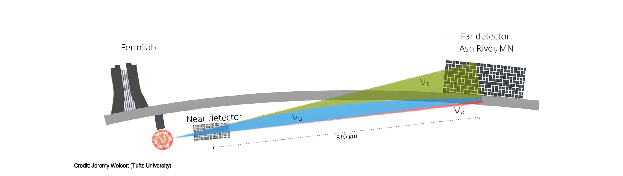
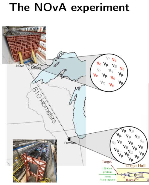
The apparatus. Two functionally identical liquid-scintillator tracking calorimeters sit in Fermilab’s NuMI beam: a near detector at Fermilab, and a 14 kt far detector 810 km away at Ash River, Minnesota. Both sit 14.6 mrad off the beam axis, and that single design choice is what makes the experiment work: going off-axis narrows the flux into a band around 2 GeV (close to the \(\nu_\mu \rightarrow \nu_e\) oscillation maximum) whilst stripping out the high-energy tail that would otherwise dominate the neutral-current background.
The underlying relation. Flavour eigenstates are superpositions of mass eigenstates, \(\lvert\nu_\alpha\rangle = \sum_i U^{*}_{\alpha i}\lvert\nu_i\rangle\), and propagating them gives the transition probability in full three-flavour form:
\[P(\nu_\alpha \to \nu_\beta) = \delta_{\alpha\beta} - 4\sum_{j>i}\mathrm{Re}\!\left[W^{ij}_{\alpha\beta}\right]\sin^{2}\!\left(\frac{\Delta m^{2}_{ji}L}{4E_\nu}\right) \pm 2\sum_{j>i}\mathrm{Im}\!\left[W^{ij}_{\alpha\beta}\right]\sin\!\left(\frac{\Delta m^{2}_{ji}L}{2E_\nu}\right)\]with \(W^{ij}_{\alpha\beta} = U_{\alpha i}U^{*}_{\beta i}U^{*}_{\alpha j}U_{\beta j}\) and \(\Delta m^{2}_{ij} = m_i^{2}-m_j^{2}\). The final term is the one that matters most here: it changes sign between neutrinos and antineutrinos, and therefore vanishes unless the mixing matrix is genuinely complex. That term is CP violation; measuring it is precisely why the experiment runs in both beam modes.
The structure is easier to read once the mixing matrix is split into the three rotations that different classes of experiment actually measure:
\[U = \underbrace{\begin{pmatrix} 1 & 0 & 0 \\ 0 & c_{23} & s_{23} \\ 0 & -s_{23} & c_{23}\end{pmatrix}}_{\text{atmospheric, NOvA}} \underbrace{\begin{pmatrix} c_{13} & 0 & s_{13}e^{-i\delta_{CP}} \\ 0 & 1 & 0 \\ -s_{13}e^{i\delta_{CP}} & 0 & c_{13}\end{pmatrix}}_{\text{reactor, Daya Bay}} \underbrace{\begin{pmatrix} c_{12} & s_{12} & 0 \\ -s_{12} & c_{12} & 0 \\ 0 & 0 & 1\end{pmatrix}}_{\text{solar, KamLAND}}\]The phase \(\delta_{CP}\) sits in the middle factor, next to \(s_{13}\); it is therefore reachable only through a channel in which \(\theta_{13}\) participates (i.e., through \(\nu_e\) appearance, not through \(\nu_\mu\) disappearance).
The measurements. Electron-neutrino appearance and muon-neutrino disappearance, in both neutrino and antineutrino beam modes. Together these constrain the mass ordering, the octant of \(\theta_{23}\), and \(\delta_{CP}\).
Disappearance is very nearly a two-flavour problem, and that is why it delivers the precision:
\[P(\nu_\mu \to \nu_\mu) \simeq 1 - \left(\cos^{4}\theta_{13}\sin^{2}2\theta_{23} + \sin^{2}2\theta_{13}\sin^{2}\theta_{23}\right)\sin^{2}\!\left(\frac{\Delta m^{2}_{32}L}{4E_\nu}\right)\]with the phase in working units,
\[\frac{\Delta m^{2}L}{4E_\nu} = 1.267\,\frac{\Delta m^{2}\,[\mathrm{eV}^{2}]\;L\,[\mathrm{km}]}{E_\nu\,[\mathrm{GeV}]}\]At \(L = 810\) km this places the first oscillation maximum at 1.6 GeV, which is exactly what the 14.6 mrad off-axis angle is chosen to sit on. The depth of the dip gives \(\sin^{2}2\theta_{23}\) and its position gives \(\lvert\Delta m^{2}_{32}\rvert\); however, a depth is symmetric about maximal mixing, so disappearance on its own cannot say whether \(\theta_{23}\) lies above or below \(45^\circ\). That is the octant degeneracy, and it is broken by combining appearance with an external constraint on \(\theta_{13}\).
Appearance carries the physics we are actually after, at the cost of being an irreducibly three-flavour problem. Expanded to second order in the small quantities \(\alpha = \Delta m^{2}_{21}/\Delta m^{2}_{31}\) and \(\sin\theta_{13}\):
\[\begin{aligned} P(\nu_\mu \to \nu_e) \;\simeq\;& \underbrace{\sin^{2}\theta_{23}\,\sin^{2}2\theta_{13}\,\frac{\sin^{2}(\Delta - aL)}{(\Delta - aL)^{2}}\,\Delta^{2}}_{\text{leading: }\theta_{13}\text{, octant, matter}} \\[2.2ex] &+ \underbrace{\alpha\,\tilde{J}\,\cos(\Delta \mp \delta_{CP})\,\frac{\sin(aL)}{aL}\,\frac{\sin(\Delta - aL)}{\Delta - aL}\,\Delta}_{\text{interference: where }\delta_{CP}\text{ lives}} \\[2.2ex] &+ \underbrace{\alpha^{2}\,\cos^{2}\theta_{23}\,\sin^{2}2\theta_{12}\,\frac{\sin^{2}(aL)}{(aL)^{2}}\,\Delta^{2}}_{\text{solar}} \end{aligned}\]where \(\Delta = \Delta m^{2}_{31}L/4E_\nu\), \(\tilde{J} = \cos\theta_{13}\sin2\theta_{12}\sin2\theta_{13}\sin2\theta_{23}\), and the upper sign is for neutrinos.
Two signs, one measurement. The term \(a = G_F N_e/\sqrt{2}\) is the matter potential: neutrinos traversing rock forward-scatter off electrons, and only \(\nu_e\) has a charged-current channel available, so the electron flavour alone picks up an extra energy
\[V = \sqrt{2}\,G_F N_e \simeq 7.56 \times 10^{-14}\,Y_e\,\rho\,[\mathrm{g\,cm^{-3}}]\ \mathrm{eV}\]\(V\) flips sign for antineutrinos, and its effect flips with the mass ordering; \(\delta_{CP}\) likewise flips sign between beam modes. These 2 sign flips and one pair of rates, as a whole, are what make the field difficult. The way out is a baseline long enough for matter to contribute materially. At 810 km and 2 GeV the matter effect moves the appearance probability by roughly 19%, against about 9% for T2K’s 295 km at 0.6 GeV. NOvA is long enough to feel the Earth; T2K is not, and that asymmetry between the two experiments is exactly why a joint fit says more than either alone.
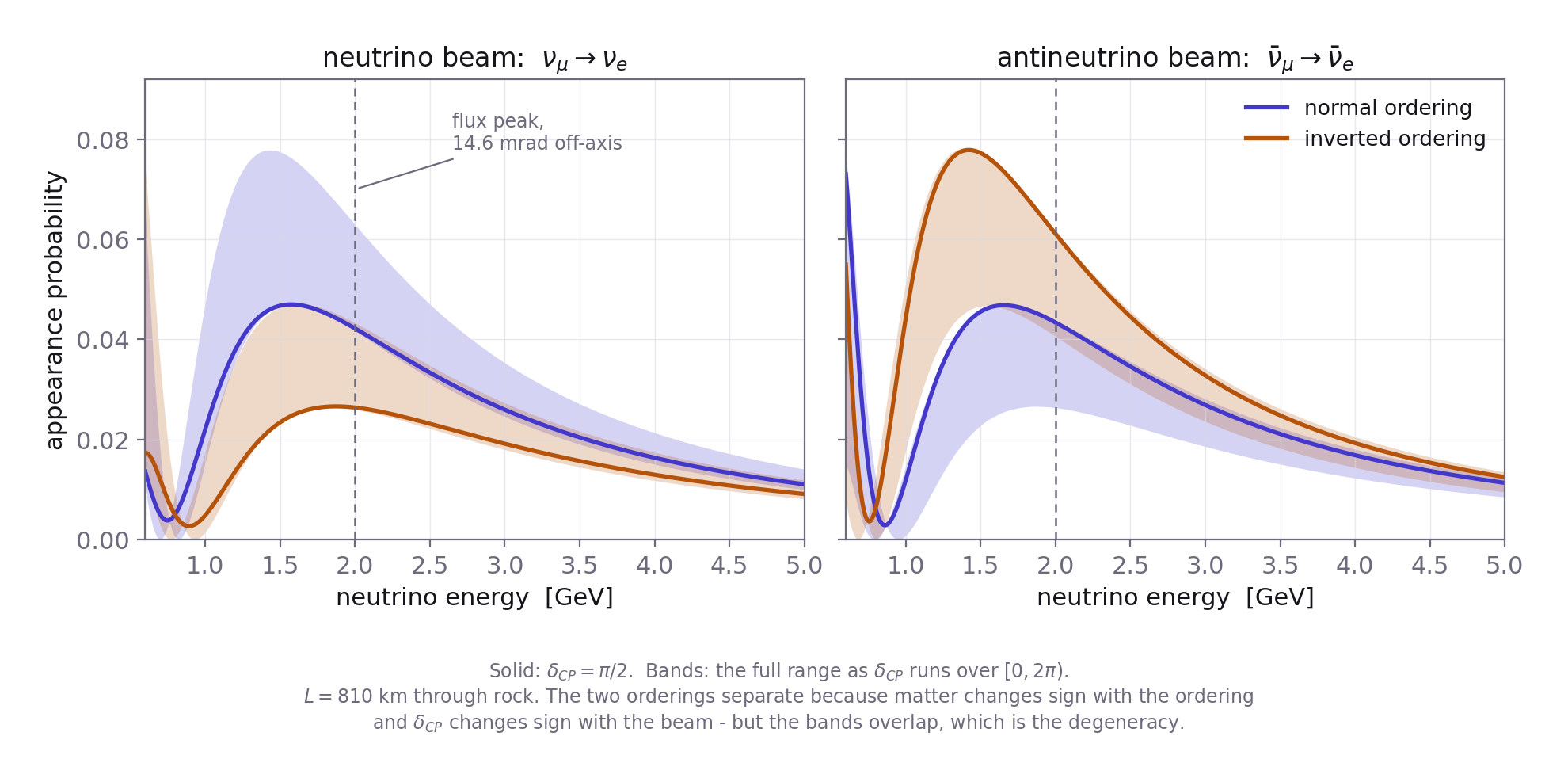
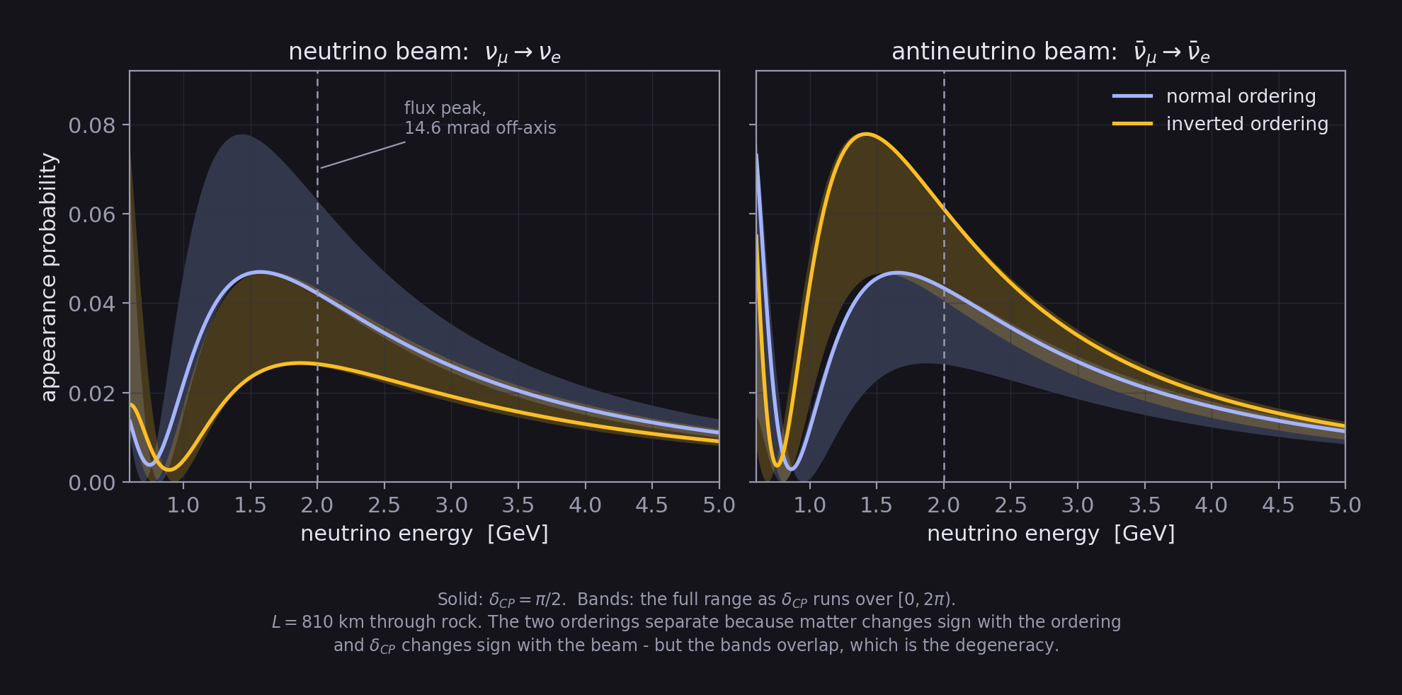
My own calculation: full three-flavour propagation through constant-density rock, at NOvA's ten-year parameter values.
The asymmetry is the observable. What the experiment actually compares is
\[\mathcal{A}_{CP} = \frac{P(\nu_\mu \to \nu_e) - P(\bar\nu_\mu \to \bar\nu_e)}{P(\nu_\mu \to \nu_e) + P(\bar\nu_\mu \to \bar\nu_e)}\]Furthermore, the genuinely CP-violating part of that asymmetry is controlled by a single parameterisation-independent number, the Jarlskog invariant:
\[J_{CP} = \tfrac{1}{8}\sin2\theta_{12}\sin2\theta_{23}\sin2\theta_{13}\cos\theta_{13}\sin\delta_{CP}\]If \(J_{CP} = 0\), the lepton sector conserves CP, whatever parameterisation one adopts. Everything NOvA does in antineutrino mode exists in order to put a number on it.
Plotting the two rates against one another makes the difficulty visible:
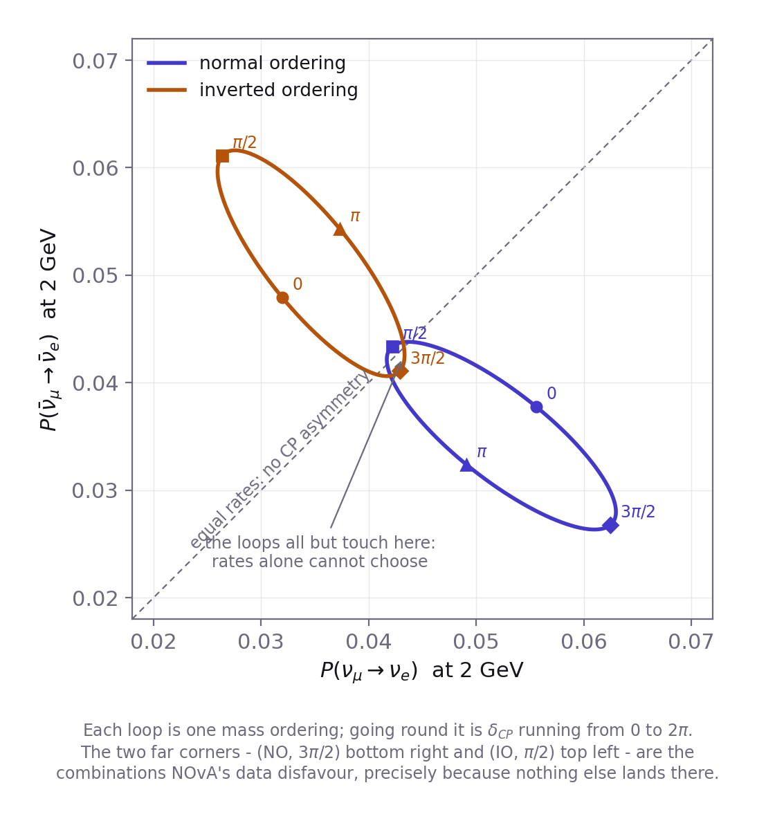
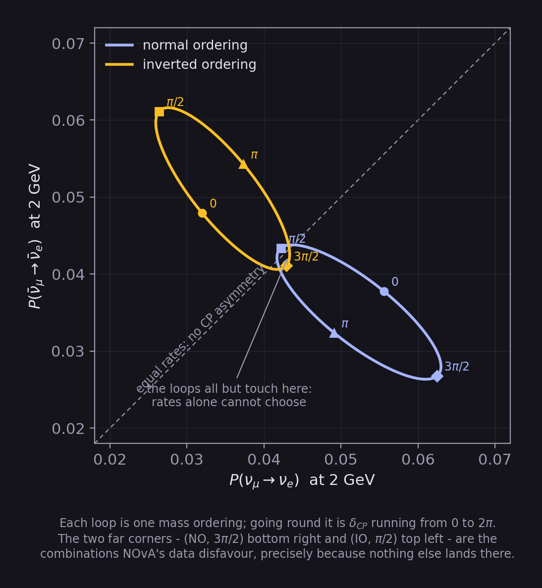
How the answer gets stated. The two orderings are discrete hypotheses rather than a parameter one fits; the result is therefore quoted as a Bayes factor, i.e., the ratio of marginal likelihoods:
\[B_{\mathrm{NO/IO}} = \frac{P(\mathbf{d}\mid \mathrm{NO})}{P(\mathbf{d}\mid \mathrm{IO})} = \frac{\int P(\mathbf{d}\mid\boldsymbol\theta,\mathrm{NO})\,\pi(\boldsymbol\theta\mid\mathrm{NO})\,d\boldsymbol\theta}{\int P(\mathbf{d}\mid\boldsymbol\theta,\mathrm{IO})\,\pi(\boldsymbol\theta\mid\mathrm{IO})\,d\boldsymbol\theta}\]Writing it out is worthwhile, because it makes the caveat visible: the integral runs over a prior, so any preference quoted for the ordering is only as defensible as the prior on \(\delta_{CP}\) underneath it. NOvA does not lean on a single fitter for precisely this reason; the collaboration runs one frequentist fit alongside two independent Bayesian ones (a Metropolis-style MCMC, and a Hamiltonian Monte Carlo implementation in Stan), and requires all three to agree before anything is published. This is the part of the experiment I work on.
Why it matters to my work. Of everything the Imperial group does, the interpretable-reconstruction strand is the one I came for. What I want to build is not merely a reconstruction network that scores well; rather, one that is systematics-aware and whose failure modes can be audited. In addition, working across several physics analyses at once is the fastest way to learn where an experiment’s systematics actually live: you watch the same nuisance parameters resurface in different measurements, which a single channel never reveals. Imperial treats NOvA and DUNE as one programme rather than two, and in practice that means the reconstruction and inference methods I develop are pressure-tested against real data, with real systematics, on NOvA before they are ever asked to carry a DUNE measurement. That is the right order in which to do it: a method that has never met a real detector is a hypothesis, not yet an instrument.
Work in progress; outputs will appear here and on Publications.
Neutrino Physics @ Imperial College London, DUNE & NOvA Collab || Machine Learning || Quantum Computing || Quant Researcher || Multidisciplinary Scientist || Physics × ML × QC × Quant || 🇬🇧 London-based (2023–Present)
Imperial College London | Imperial College London
View profile